Using the Galvo Calibration File Converter with the Automation1-GI4

Calibrating the field of view for scanners is typically an iterative process where a series of marks are placed on a substrate and the location of these marks is used to create a calibration file, and the process is repeated to reach final system accuracy. Each iteration of the mark and measure sequence must combine the new measurement values with the current calibration table to create a new calibration table. When the tables are of the same resolution, the values can be added directly to each other. When the density of the marks in the tables to be combined is not equal, an algorithm must be applied to interpolate lower resolution data with higher resolution data.

Aerotech’s Galvo Calibration File Converter (GCFC) application can be used to merge measurement data during the calibration process. The measurement resolutions of the tables to be merged do not have to match as GCFC will interpolate the correction values of the lower resolution table to match those of the higher resolution table.

This application note will outline the procedures required to create new calibration tables and how to merge calibration tables for Automation1-GI4.

Calibration File Creation Process

When creating tables through a manual measurement procedure, users will typically start by marking a low resolution grid (e.g., 3 x 3), measure the placement accuracy of the grid and use the measured data to create a calibration table. The calibration table is activated and the measurement grid size is increased (e.g., 5 x 5). This sequence is repeated until the desired results are attained over the entire working area of the scanner.

For applications where the measurement of galvo accuracy is automated, the grid spacing can start at a much higher resolution (e.g., 33 x 33) since the process does not require manual measurement of the placement error at each location in the grid.

Manual File Creation Process

Step 1: Create a New File

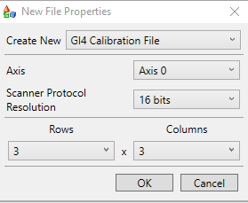
Tables should be created with an odd number of rows and columns. This is done so that there are correction values that pass through the origin (X=0, Y=0) of the scanner. To create a new file, select “New” from the “File” menu.

The “Calibration File Type” window will be displayed (Figure 1). Select the desired number of rows and columns. The table can have a different number of rows and columns. The GCFC application will interpolate the table size to 65 x 65 before saving the results to a .cal file.

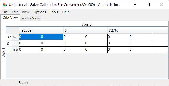
A table will be displayed with “0” correction values in all locations:

Legacy Product Consideration (Optional): Set‐Up Scaling

The following section’s content applies when you are working with a *.gcal calibration file for an Nmark SSaM. This capability currently does not apply when working with an Automation1-GI4 *.cal file.

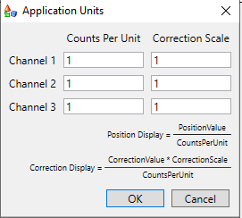
By default, all positions and correction values are displayed in counts where ‐32768 to 32767 are the full‐scale displacement of the mirrors in the scanner. The scaling can be changed to reflect user units for both the position and correction value. Select the “Change Units” item from the “Options” menu to display the Application Units dialog (Figure 3). The “Counts Per Unit” value should be set to the same value as the Automation1 CountsPerUnit axis parameter. This scale factor is used to display the measurement locations on the grid. The Application Units setting allows for the correction units to be different from the measurement units. The “Counts Per Unit” could be set‐up to reflect mm and the Correction Scale can be set‐up for microns. This allows the data to be entered into the table in more intuitive user units rather than scanner counts.

Regardless of the values used for scaling the position display and correction display, the CSV and .cal values are always stored in counts when the files are saved.

Step 2: Create the Correction Table

By default, the table elements are assumed to be “corrections” and are always stored in the CSV or .cal file as corrections. A correction is a value that is added to the commanded position to arrive at the desired position.

Position_modified = Position_command + CorrectionValue

The values can also be entered/displayed as „errors“. This value is subtracted from the commanded position to arrive at the desired position.

Position_modified = Position_command – Error

Setting of “Correction” versus “Error” is done through the “Show Values As” menu item on the “View” Menu.

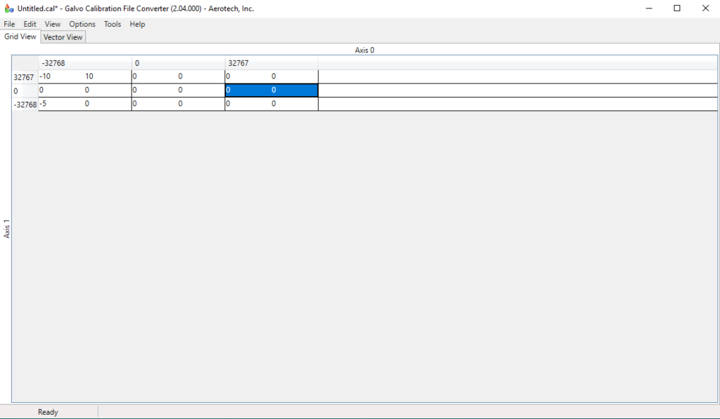
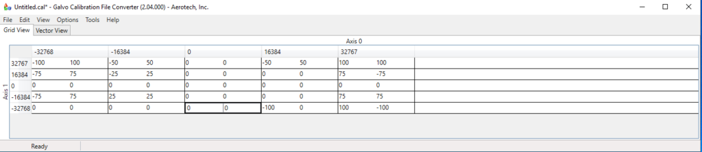
Once the correction field type is specified, the values are entered into the table by double clicking on the desired table element and typing in the value. Figure 4 is an example 3 x 3 table filled with correction values.

Save the table as “3×3.CSV” before continuing by selecting the “Save” or “Save As” menu item from the File menu with the file type set to “CSV”.

Step 3: Create and Activate an Automation1-GI4 Correction File

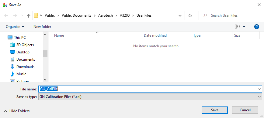
To create a Automation1-GI4 Calibration file, select the “Save As” menu item from the “File” menu, set the type as “Aerotech calibration files (*.cal)” and enter in a file name (Figure 5).

The GCFC will automatically interpolate the table to a 65 x 65 resolution table. The display will be updated to show the results of this interpolation (Figure 6).

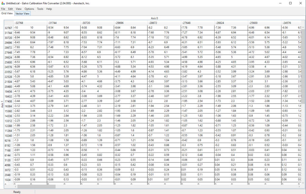
After creating and saving the higher resolution, 65×65 file, it needs to be activated on the controller. The .cal file is activated on the Automation1 controller using the Calibration module of the Configure workspace from within Automation1 Studio. See the Automation1 Help file for additional information on this process. Make sure the AeroBasic program used to create the grid test pattern is modified to use the newly created .cal file before continuing.

Step 4: Create a Higher Resolution Table

After the new .cal file is activated, mark a new grid pattern at a higher resolution. For this example, we started with 3 x 3 and will increase to 5 x 5 for the second pattern (see Step 1 for instructions on creating a new correction table). Mark and measure a 5 x 5 pattern and create a new table per the process defined in Step 3. Save this table as a CSV file.

Step 5: Merge the 3 x 3 and 5 x 5 Tables

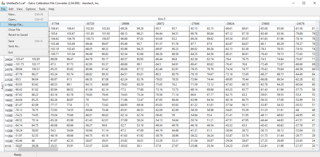
We now have two CSV files, one at 3 x 3 and the other at 5 x 5. The 3 x 3 correction table was active when the 5 x 5 was created so the correction values in the 5 x 5 table need to be merged with those from the 3 x 3 table. The tables are merged by selecting the “Merge File” menu item on the “File” menu. The currently opened file in GCFC will be merged with the selected file. With the “5×5.CSV” file open in the GCFC, select the “3X3.CSV” for merging by clicking on the “Merge File” menu item. Save this file as a new CSV file “5X5merged.CSV”, so that it can be used to create a new .cal file and for use in subsequent merging operations.

Step 6: Repeat as Required

Repeat steps 2 through 5, increasing the table size for each iteration, until the desired results are obtained.

Automated Calibration Process

The GCFC can import CSV files (Comma Separated Values) that contain the results of an automated measurement process. For example, a camera can acquire the marks made by the scanner on the substrate, measure the placement accuracy and store the results directly into a CSV file. The CSV file can be converted into a .cal file by the GCFC for use by the Automation1-GI4.

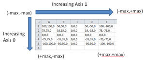
When creating the CSV file, be aware that the order of the correction elements in the CSV file differs from the Grid View; Axis 0 positions increase top to bottom and Axis 1 positions increase left to right (Figure 9).

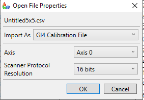
When a CSV file is opened, the user must specify the “Calibration File Type” data as “GI4 Calibration File” (Figure 10).

After opening the CSV file, the data can be saved as a 2D calibration file using the “Save As” option of the “File” menu with the file type set as “GI4 Calibration File”.